2023. 11. 2. 16:19ㆍML&DL/NLP
정수 인코딩
- 토큰화 수행 후 각 단어에 고유한 정수를 부여해주는 것
- 정수로 만드는 이유는 컴퓨터가 이해하기 쉽도록 텍스트 -> 숫자로 표현
- 모든 단어의 집합(Vocabulary)을 만들고 이를 기반으로 문서를 정수로 인코딩 해줌
패딩
- 텍스트에 대해 정수 인코딩을 수행했을 때 길이가 서로 다르게 되는데 길이를 맞춰주기 위해 사용
- 길이를 맞춰줌으로써 병렬 연산을 할 수 있게 만들어줌.
- 패딩 길이가 너무 작으면 데이터 손실의 문제, 길이가 너무 길면 중요도가 낮은 데이터 포함되는 문제가 있으므로 적절하게 지정해줘야함
💻 정수 인코딩 실습
라이브러리 불러오기
import pandas as pd
import numpy as np
import matplotlib.pyplot as plt
import nltk
import torch
import urllib.request
from tqdm import tqdm
from collections import Counter
from nltk.tokenize import word_tokenize
from sklearn.model_selection import train_test_splitnltk.download('punkt')
데이터 불러오기
- IMDB Dataset (영화 리뷰 데이터) 사용
- https://www.kaggle.com/datasets/lakshmi25npathi/imdb-dataset-of-50k-movie-reviews/
IMDB Dataset of 50K Movie Reviews
Large Movie Review Dataset
www.kaggle.com
데이터 확인
- 리뷰 내용 기반으로 두 개의 클래스로 나누어져있음 (positive/negative)

df.info()결측값 여부 : False
- 결측값 확인
print('결측값 여부 :',df.isnull().values.any())
- 클래스 불균형 확인
df['sentiment'].value_counts().plot(kind='bar')
print('레이블 개수')
print(df.groupby('sentiment').size().reset_index(name='count'))
레이블 개수
sentiment count
0 negative 25000
1 positive 25000
Train / Test dataset 분리
* stratify=y_data 옵션을 주면 비율을 균일하게 나눠줌
X_train, X_test, y_train, y_test = train_test_split(X_data, y_data, test_size=0.5, random_state=0, stratify=y_data)print('--------훈련 데이터의 비율-----------')
print(f'긍정 리뷰 = {round(y_train.value_counts()[0]/len(y_train) * 100,3)}%')
print(f'부정 리뷰 = {round(y_train.value_counts()[1]/len(y_train) * 100,3)}%')
print('--------테스트 데이터의 비율-----------')
print(f'긍정 리뷰 = {round(y_test.value_counts()[0]/len(y_test) * 100,3)}%')
print(f'부정 리뷰 = {round(y_test.value_counts()[1]/len(y_test) * 100,3)}%')
--------훈련 데이터의 비율-----------
긍정 리뷰 = 50.0%
부정 리뷰 = 50.0%
--------테스트 데이터의 비율-----------
긍정 리뷰 = 50.0%
부정 리뷰 = 50.0%'
단어 토큰화
def tokenize(sentences):
  tokenized_sentences = []
  for sent in tqdm(sentences):
    tokenized_sent = word_tokenize(sent)
    tokenized_sent = [word.lower() for word in tokenized_sent]
    tokenized_sentences.append(tokenized_sent)
  return tokenized_sentences
tokenized_X_train = tokenize(X_train)
tokenized_X_test = tokenize(X_test)
* 토큰화 결과
word_list = []
for sent in tokenized_X_train:
    for word in sent:
      word_list.append(word)

word_counts = Counter(word_list)
print('총 단어수 :', len(word_counts))
총 단어수 : 112946
* 빈도수
print(word_counts)Counter({'the': 332140, ',': 271720, '.': 234036,'and': 161143, 'a': 161005, 'of': 144426, 'to': 133327, ' .....
=> 단어별로 빈도수 출력, the가 332140번으로 가장 많이 나왔음
vocab = sorted(word_counts, key=word_counts.get, reverse=True)
print('등장 빈도수 상위 10개 단어')
print(vocab[:10])
['the', ',', '.', 'and', 'a', 'of', 'to', 'is', '/', '>']
단어 집합(vocabulary) 사이즈 줄이기
- 빈도수가 낮은 단어는 배제
* threshold = 3
=> 3번 미만으로 나온 단어들 카운트
threshold = 3
total_cnt = len(word_counts) # 단어의 수
rare_cnt = 0 # 등장 빈도수가 threshold보다 작은 단어의 개수를 카운트
total_freq = 0 # 훈련 데이터의 전체 단어 빈도수 총 합
rare_freq = 0 # 등장 빈도수가 threshold보다 작은 단어의 등장 빈도수의 총 합

# 단어와 빈도수의 쌍(pair)을 key와 value로 받는다.
for key, value in word_counts.items():
    total_freq = total_freq + value

    # 단어의 등장 빈도수가 threshold보다 작으면
    if(value < threshold):
        rare_cnt = rare_cnt + 1
        rare_freq = rare_freq + value

print('단어 집합(vocabulary)의 크기 :',total_cnt)
print('등장 빈도가 %s번 이하인 희귀 단어의 수: %s'%(threshold - 1, rare_cnt))
print("단어 집합에서 희귀 단어의 비율:", (rare_cnt / total_cnt)*100)
print("전체 등장 빈도에서 희귀 단어 등장 빈도 비율:", (rare_freq / total_freq)*100)
단어 집합(vocabulary)의 크기 : 112946
등장 빈도가 2번 이하인 희귀 단어의 수: 69670
단어 집합에서 희귀 단어의 비율: 61.68434473111044
전체 등장 빈도에서 희귀 단어 등장 빈도 비율: 1.1946121064938062
=> 전체 단어 집합 크기가 112946개 인데 2번 이하로 나온 단어가 무려 69670개나 된다. 중요하지 않은 단어는 삭제할 필요가 있음
* 빈도수 낮은 단어 제거
# 전체 단어 개수 중 빈도수 1이하인 단어는 제거.
vocab_size = total_cnt - rare_cnt
vocab = vocab[:vocab_size]
print('단어 집합의 크기 :', len(vocab))
단어에 정수 매핑 해주기
- <PAD> 와 <UNK> 를 0, 1 로 매핑해준 후 등장 빈도수가 가장 높은 the 부터 차례대로 숫자를 부여
* <PAD> => 인코딩 후 단어 길이를 맞춰주기 위한 용도로 사용
* <UNK> => 단어 집합에 없는 단어가 나왔을 때 사용
word_to_index = {}
word_to_index['<PAD>'] = 0
word_to_index['<UNK>'] = 1
for index, word in enumerate(vocab) :
word_to_index[word] = index + 2print(word_to_index)
{'<PAD>': 0, '<UNK>': 1, 'the': 2, ',': 3, '.': 4, 'and': 5, 'a': 6, 'of': 7, 'to': 8, 'is': 9, '/': 10, '>': 11, '<': 12, 'br': 13, 'it': 14, 'in': 15, 'i': 16, 'this': 17, 'that': 18, "'s": 19, 'was': 20, 'as': 21, 'with': 22, 'for': 23, ' ….'questionmark.': 43274, '-atlantis-': 43275, 'middlemarch': 43276, 'lollo': 43277}
=> 0 부터 43277 까지 빈도수 순서대로 매핑된 것을 확인할 수 있음
정수로 인코딩된 데이터를 저장해주기
- encoded_X_train, encoded_X_test에 저장
def texts_to_sequences(tokenized_X_data, word_to_index):
  encoded_X_data = []
  for sent in tokenized_X_data:
    index_sequences = []
    for word in sent:
      try:
          index_sequences.append(word_to_index[word])
      except KeyError:
          index_sequences.append(word_to_index['<UNK>'])
    encoded_X_data.append(index_sequences)
  return encoded_X_data
encoded_X_train = texts_to_sequences(tokenized_X_train, word_to_index)
encoded_X_test = texts_to_sequences(tokenized_X_test, word_to_index)
- 토큰화 후 인코딩 X 상태와 토큰화 후 인코딩 O 상태 비교
print('인코딩 전',tokenized_X_train[0])
print('인코딩 후', encoded_X_train[0])
인코딩 전 ['life', 'is', 'too', 'short', 'to', 'waste', 'on', 'two', 'hours', 'of', 'hollywood', 'nonsense', 'like', 'this', ',', 'unless', 'you', "'re", 'a', 'clueless', 'naiive', '16', 'year', 'old', 'girl', 'with', 'no', 'sense', 'of', 'reality', 'and', 'nothing', 'better', 'to', 'do', '.', 'dull', 'characters', ',', 'poor', 'acting', '(', 'artificial', 'emotion', ')', ',', 'weak', 'story', ',', 'slow', 'pace', ',', 'and', 'most', 'important', 'to', 'this', 'films', 'flawed', 'existence-no', 'one', 'cares', 'about', 'the', 'overly', 'dramatic', 'relationship', '.']
인코딩 후 [139, 9, 117, 353, 8, 459, 30, 129, 635, 7, 360, 1934, 50, 17, 3, 898, 29, 192, 6, 5485, 1, 4041, 346, 188, 261, 22, 72, 307, 7, 605, 5, 176, 143, 8, 54, 4, 772, 119, 3, 351, 132, 28, 4786, 1386, 27, 3, 838, 81, 3, 617, 1057, 3, 5, 104, 681, 8, 17, 123, 2958, 1, 40, 1994, 57, 2, 2346, 950, 632, 4]
💻 패딩 실습
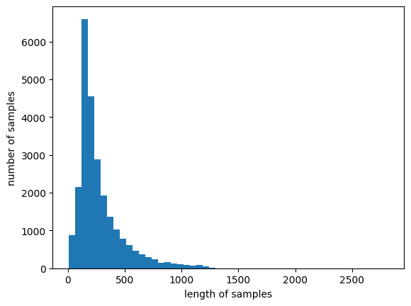
* 데이터 길이 확인
print('리뷰의 최대 길이 :',max(len(review) for review in encoded_X_train))
print('리뷰의 평균 길이 :',sum(map(len, encoded_X_train))/len(encoded_X_train))
plt.hist([len(review) for review in encoded_X_train], bins=50)
plt.xlabel('length of samples')
plt.ylabel('number of samples')
plt.show()
리뷰의 최대 길이 : 2818
리뷰의 평균 길이 : 279.0998
def below_threshold_len(max_len, nested_list):
  count = 0
  for sentence in nested_list:
    if(len(sentence) <= max_len):
        count = count + 1
  print('전체 샘플 중 길이가 %s 이하인 샘플의 비율: %s'%(max_len, (count / len(nested_list))*100))
max_len = 500
below_threshold_len(max_len, encoded_X_train)전체 샘플 중 길이가 500 이하인 샘플의 비율: 87.836
* max_len = 500
- 500보다 길이가 짧다면 0을 채워서 500으로 만들고, 500보다 길다면 뒷부분은 잘라서 500으로 만들어줌
def pad_sequences(sentences, max_len):
  features = np.zeros((len(sentences), max_len), dtype=int)
  for index, sentence in enumerate(sentences):
    if len(sentence) != 0:
      features[index, :len(sentence)] = np.array(sentence)[:max_len]
  return features
* 패딩 작업
def pad_sequences(sentences, max_len):
  features = np.zeros((len(sentences), max_len), dtype=int)
  for index, sentence in enumerate(sentences):
    if len(sentence) != 0:
      features[index, :len(sentence)] = np.array(sentence)[:max_len]
  return features
padded_X_train = pad_sequences(encoded_X_train, max_len=max_len)
padded_X_test = pad_sequences(encoded_X_test, max_len=max_len)
print('훈련 데이터의 크기 :', padded_X_train.shape)
print('테스트 데이터의 크기 :', padded_X_test.shape)
훈련 데이터의 크기 : (25000, 500)
테스트 데이터의 크기 : (25000, 500)

'ML&DL > NLP' 카테고리의 다른 글
| [NLP] 텍스트 벡터화 : TF-IDF 실습 (1) | 2023.11.03 |
|---|---|
| [NLP] 텍스트 벡터화 (0) | 2023.11.03 |
| [NLP] 데이터 전처리 - 정제 / 정규화 (0) | 2023.09.27 |
| [NLP] 데이터 전처리 - 영어/ 한국어 토큰화 실습 (0) | 2023.09.21 |
| [NLP] 데이터 전처리 - 한국어 토큰화 (0) | 2023.09.21 |